
3. Your first workflow
Watch the 8 walkthrough videos for this chapter
You will build one small data product from start to finish. Each step uses what the one before it made, and ends with something you can see.
What you need for this chapter
Permission to add connections, to create datasets, visualizations and dashboards, to create projects and run ETL jobs, and to use a compute size. If a step is refused, the message tells you which permission to ask for.
The examples use a PostgreSQL connection called acme-postgres (the storefront database) and a Lakehouse connection called acme-lakehouse. Use your own names wherever you see them.
Step 1: Connect a data source#
Why: Everything else in this guide reads from a connection. When you finish this step, you have a saved link to your data that you can reuse.
Open Connections in the top bar. The page lists every connection you can see, with its type, a category (for example Lakehouse, Database or Object storage), who updated it and when. Use the search box and the Type, Owner and Updated filters to find one.
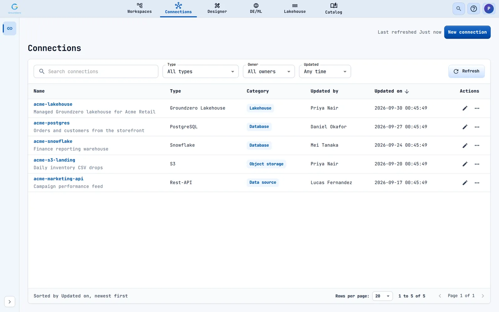
To add a connection:
- Choose New connection. The Add Connection dialog opens.
- Open Connection Type and choose your source. The list is alphabetical and includes databases, warehouses, object stores, streaming systems, business applications, AI providers and the Groundzero Lakehouse. Type to search it.
- Fill in the form that appears. A PostgreSQL connection asks for Connection Name, Port, Server, Username, Database and Password.
- Choose Test Connection. A green message confirms that Groundzero can reach the source. Testing saves nothing.
- Choose Save.

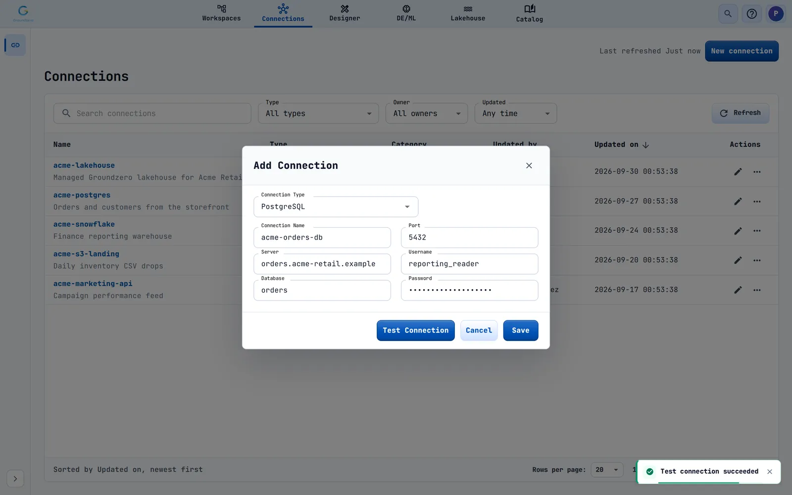
What you should see: The message Connection created successfully, and your connection in the list.
Naming a connection
A connection name starts with a letter and uses only letters, numbers and single hyphens, for example acme-postgres. A bad name is rejected when you choose Save.
Secrets stay hidden
Choose a connection's name to see its Configured details. Passwords, tokens and keys appear as hidden values. Your code and datasets use the connection by name and never see the credentials.
If something goes wrong: If Test Connection and Save stay greyed out, a field is empty. Fill in every field.
Step 2: Explore it in the Catalog#
Why: Before you build on data, check what it is. The Catalog is also where colleagues, and the AI assistant, look first. When you finish this step, you have found an item and described it.
Open Catalog in the top bar. The Catalog lists three kinds of things: Datasets, Jobs (ETL jobs) and Warehouses (lakehouse warehouses). You can change only descriptions and tags here. Warehouses appear only if you may list them.
- Type in Search catalog, or choose All, Datasets, Jobs or Warehouses to narrow the list.
- Select an item. Its header shows the type, owner and last update, with an Open button that takes you to the item itself.
- On the Overview tab, read or edit the Description. You can write it yourself or choose Draft with AI. Add Tags too.
- For datasets and jobs, the Contract tab shows how to call the item from outside Groundzero.
- Select a warehouse and open its Schema tab to browse databases, tables and columns, with their sizes and tags.


What you should see: The description and tags you saved on the item's Overview tab.
Good descriptions pay off
Add a one-sentence description to everything you publish. It is what colleagues find first.
Step 3: Build a dataset#
Why: Charts and dashboards read datasets, so a good dataset is the foundation for everything after it. When you finish this step, you have a saved query that returns the rows you want.
- Open Designer. The left menu has Datasets, Filters, Visualizations and Dashboards. Choose Datasets.
- Choose New Dataset, type a name such as
acme-weekly-salesin Enter Name and choose Add. - Open the new dataset from the list. The editor opens with the Query and Prep tabs.
- In the left drawer, open Connections and tick the connection to query, for example
acme-postgres. It expands into databases, tables and columns that you can browse. - On the Query tab, write your SQL. The editor suggests connection, table and column names as you type.
- Leave the runtime picker on Standard. Standard runs one SQL query straight against the source and needs no compute size.
- Choose Run (the play button). Results shows the response time, the row count, the page size and the rows, with each column's data type. Messages shows success or the error text.
- Choose Save (the disk button).


SELECT category, revenue, units_sold, avg_discount_pct
FROM sales.category_summary
WHERE year = 2025
What you should see: Rows under Results after you run the query, and the message Dataset updated after you save.
Let the assistant help
The sparkle button in the toolbar (Generate code with GZ) opens a code assistant that knows this dataset. Describe the query you want, review what it writes, and run it. Chapter 5 has more.
Good to know
Standard works with SQL connections such as PostgreSQL, MySQL, SQL Server, Oracle, Snowflake, Redshift, Google BigQuery and the Groundzero Lakehouse. If you choose another runtime, or more than one connection, the dataset becomes a code dataset that you write in Python on the Prep tab. Groundzero keeps the results of an identical query in your browser for 10 minutes, so reload the page if you want a fresh start.
If something goes wrong: If Run says Please select Connection, tick a connection in the left drawer first.
Step 4: Create a visualization#
Why: A chart makes a result easy to read at a glance. When you finish this step, you have a saved chart on your dataset.
- In Designer, choose Visualizations, then New Visualization. Enter a name such as
revenue-by-categoryand choose Add. Groundzero does not open it for you, so choose its name in the list. - In the Setup tab on the right, open Chart Type and choose a type. Hover over an icon to see its name. There are 22 types: Bar, Vertical Bar, Stacked Bar, Stacked Vertical Bar, Combo, Line, Pie, Half Donut, Donut, Gauge, Bubble, Scatter, Candle, Tree Map, Geo, Funnel, Table, Pivot, Sunburst, Sankey, Card and Graph.
- In Choose Dataset, pick the dataset from step 3.
- Map columns to the roles of the chart. A bar chart asks for a vertical axis (the category) and a series (the measure, here
revenue). Add a Chart Title. - Open Customize to style the chart: axes and titles, colours, legends and labels.
- Choose the Save icon (the disk at the top right). Groundzero does not save automatically, so save before you leave.
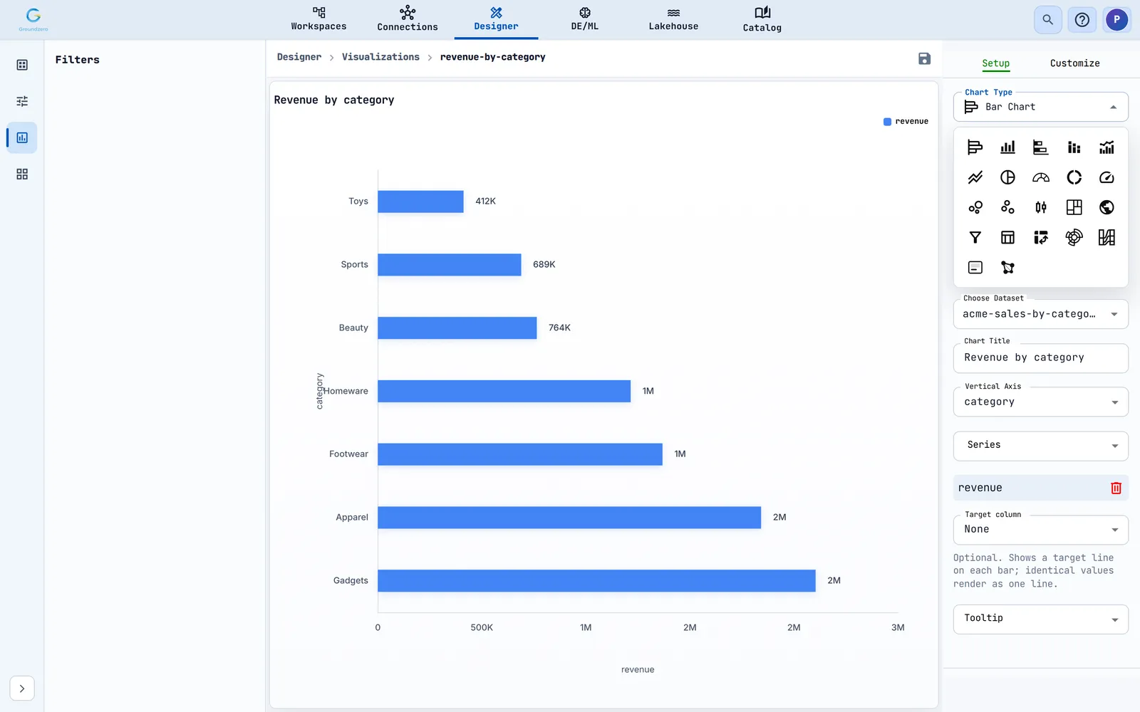
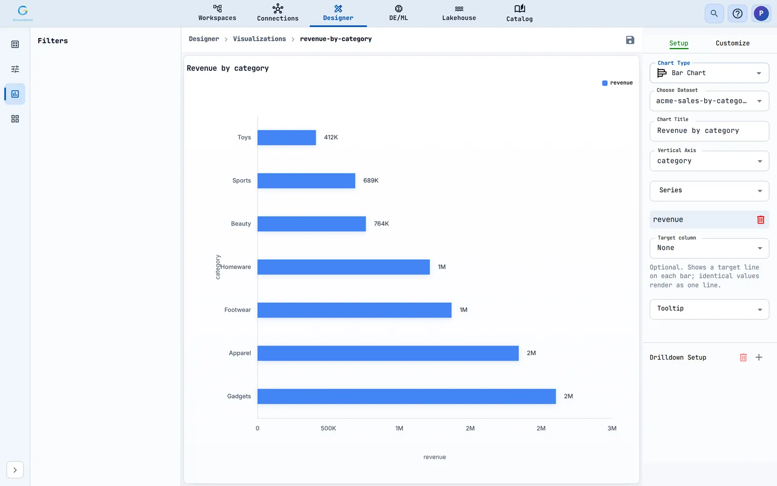
What you should see: Your chart, drawn from the dataset's rows.
Charts always show current data
Groundzero saves the design of your chart, not its rows. It runs the dataset again every time the chart opens, so a saved chart is always up to date.
Step 5: Compose and publish a dashboard#
Why: A dashboard puts several charts on one page, and publishing lets other people open it. When you finish this step, your chart is on a dashboard in a workspace folder.
- In Designer, choose Dashboards, then New Dashboard. Name it with the usual rule, for example
Acme-Sales-Overview, and choose Add. Open it from the list. - In the right panel, choose the first icon, Select visualizations. Tick the visualizations to add. Each one becomes a tile on the canvas. Drag a tile to move it, and drag its edge to resize it. Untick a visualization to remove its tile.
- Use the tabs at the bottom to organise the dashboard. Choose + to add a tab, and use the menu beside a tab name to rename, duplicate or delete it.
- The Setup tab holds Triggers (click a chart to filter other charts or jump to another tab), Text and Shapes and Dashboard Filters. The Customize tab styles tiles, text and backgrounds.
- Choose Save dashboard (the disk icon at the top right).
- Choose Publish and confirm. Publishing makes the dashboard available to import into a workspace.
- Open Workspaces, choose a folder, choose Import Dashboard, pick the published dashboard and choose Import.


What you should see: The dashboard in the workspace folder. Open it from there to read it.
Save first, then publish
Publish does not save your changes. It publishes the last saved version, and it replaces a published dashboard that has the same name. Choose Save dashboard and then Publish.
Taking a dashboard with you
The export button in the dashboard header offers Export To PDF and Export to Excel. Each export covers the tab you are on.
If something goes wrong: If you see Dashboard is empty, add some items and save., add at least one visualization first.
Step 6: Automate with a job and a schedule#
Why: A dataset answers a question when you ask it. A job prepares and moves data without you, for example every morning, so the data behind your dashboard stays current. Jobs live in a project. When you finish this step, you have a job that runs by itself every day.
Create a project
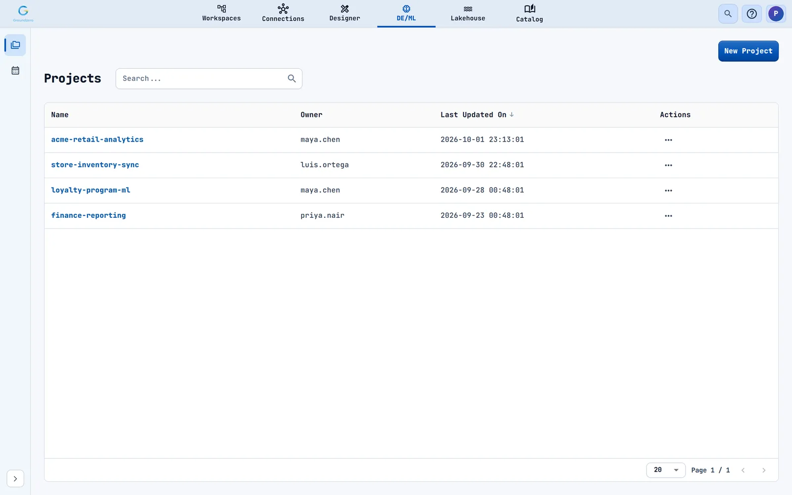
- Open DE/ML. The Projects page lists your projects with their owner and last update.
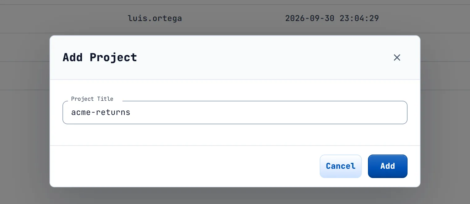
- Choose New Project, enter a Project Title (the usual name rule), and choose Add.
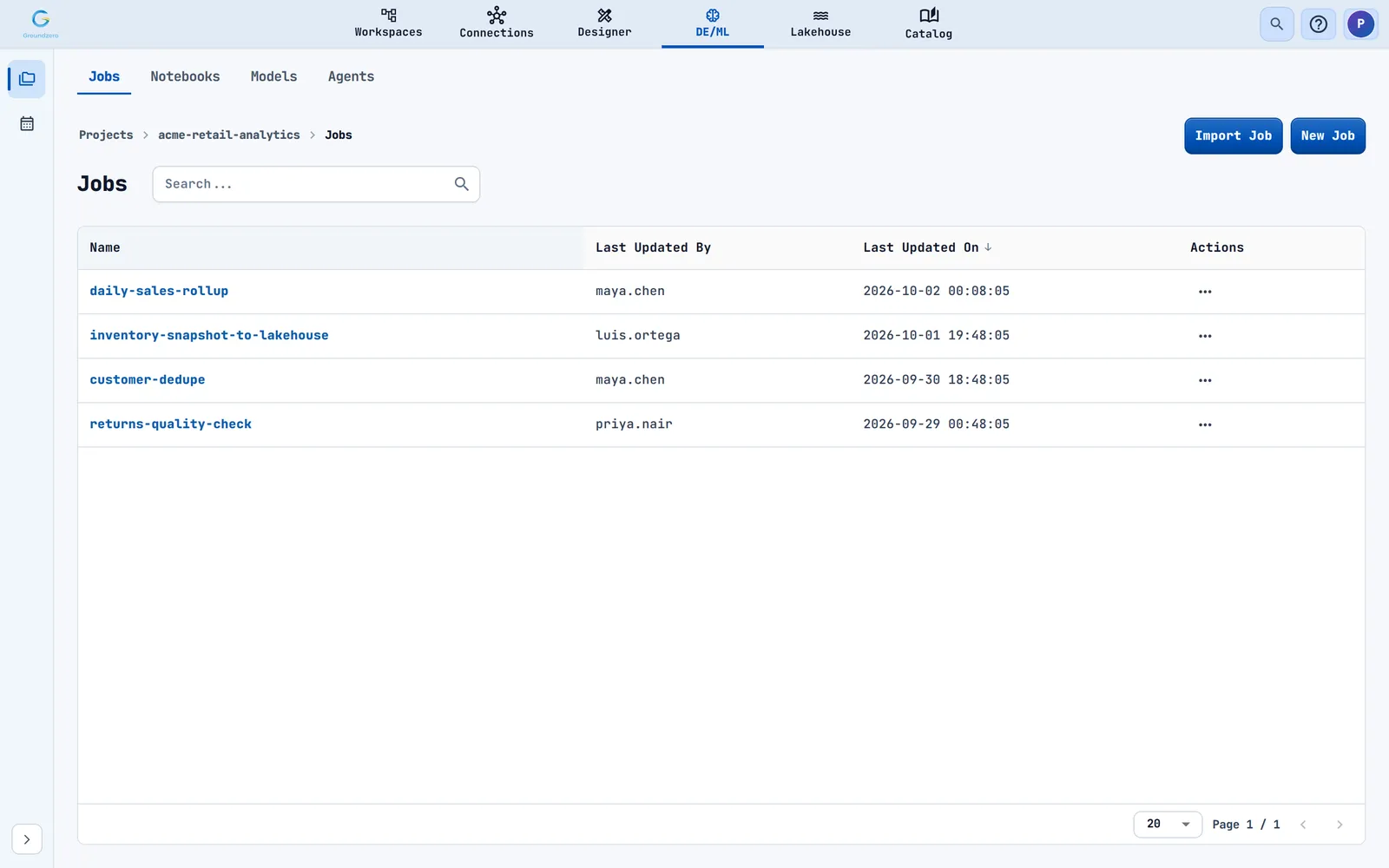
- Choose the project name. Its tabs are Jobs, Notebooks, Models and Agents.
Create and run a job
- On the Jobs tab, choose New Job, enter a Job Title such as
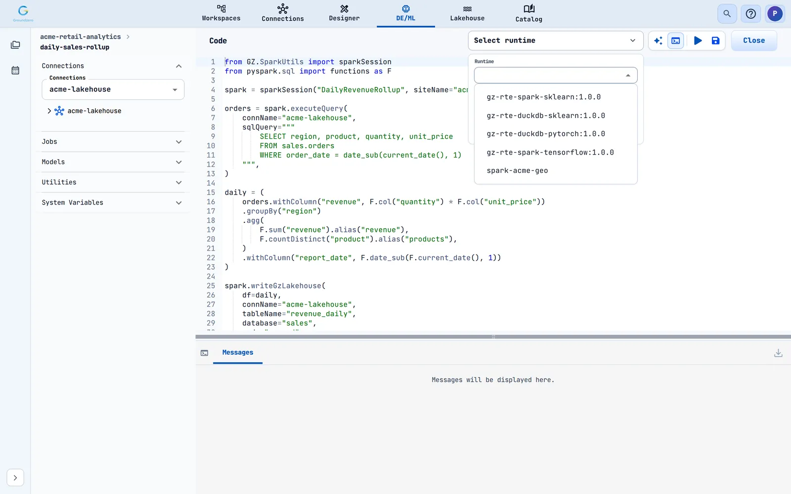
daily-sales-rollupand choose Add. - Choose the job name to open the editor. In the left drawer, tick the Connections the job uses. Your code can use only the connections you tick.
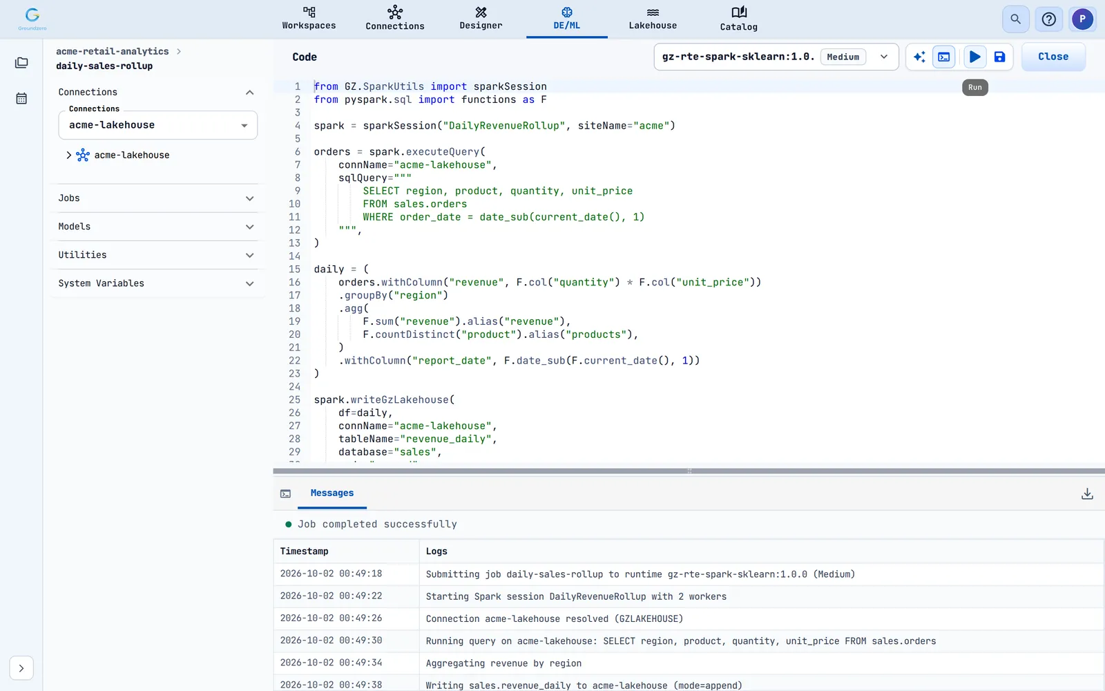
- Write the Python code. Jobs run on a Spark or DuckDB runtime. The example below reads yesterday's orders from the lakehouse, adds them up by region and appends the result to a table.
- Open the runtime picker in the toolbar. Choose a Runtime and a Compute size, then close the panel.
- Choose Run. The Messages pane shows the log while the job runs and ends with the job status. Choose Save when you are happy with the job.

from GZ.SparkUtils import sparkSession
from pyspark.sql import functions as F

spark = sparkSession("DailyRevenueRollup", siteName="acme")

orders = spark.executeQuery(
    connName="acme-lakehouse",
    sqlQuery="""
        SELECT region, product, quantity, unit_price
        FROM sales.orders
        WHERE order_date = date_sub(current_date(), 1)
    """,
)

daily = (
    orders.withColumn("revenue", F.col("quantity") * F.col("unit_price"))
    .groupBy("region")
    .agg(
        F.sum("revenue").alias("revenue"),
        F.countDistinct("product").alias("products"),
    )
    .withColumn("report_date", F.date_sub(F.current_date(), 1))
)

spark.writeGzLakehouse(
    df=daily,
    connName="acme-lakehouse",
    tableName="revenue_daily",
    database="sales",
    mode="append",
)

outputDF = daily.orderBy(F.desc("revenue"))
What you should see: Job completed successfully at the end of the log.
Why outputDF?
When your script finishes, Groundzero looks for a variable named outputDF at the top level of your code. A Spark DataFrame, a pandas DataFrame or a list of dictionaries works. If it is missing, the job still succeeds but shows no preview.
Schedule the job
Open DE/ML, then choose the calendar icon in the left menu (Scheduler).
- Choose New Task.
- Choose Select Project and Select Job.
- Choose the RTE box, pick a Runtime and a Compute size, and choose Save in the panel.
- Choose Batch for a repeating schedule. Streaming, the default, runs the job once.
- Type a Name (letters, digits, dot, hyphen and underscore; no spaces) and pick the Start date and Start time.
- Under Recurrence, set Repeat (Minutes, Hourly, Daily, Weekly, Monthly or Yearly) and Ends (Never or On a date).
- Choose Save.

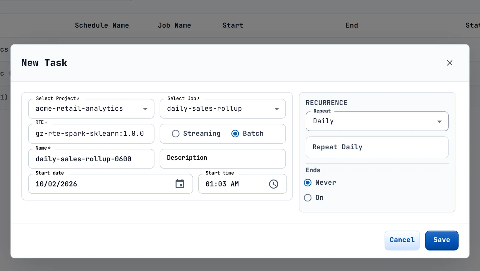
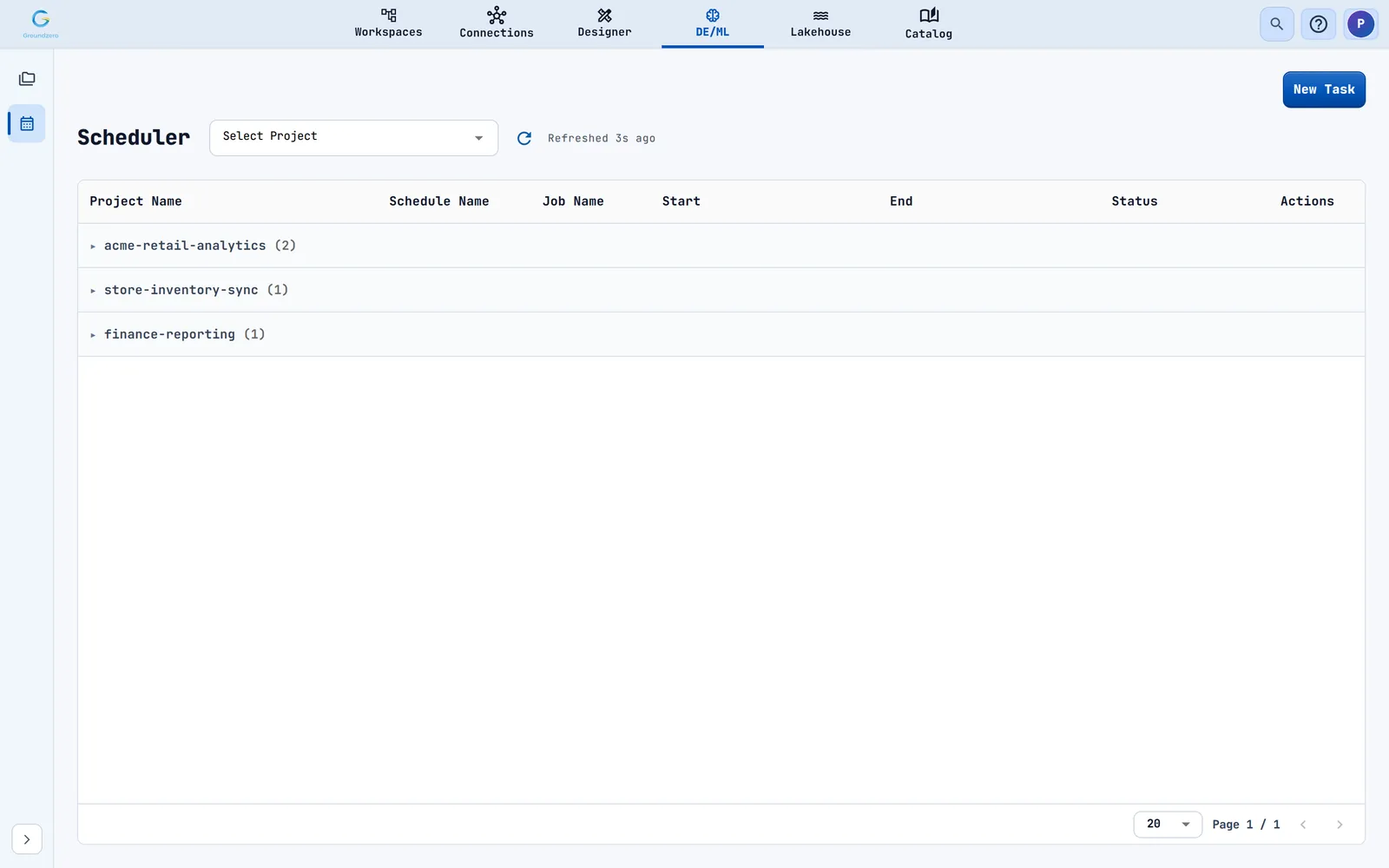
What you should see: The message Job scheduled successfully, and your task in the Scheduler. Choose Run Once on its menu to check that it works without waiting, then View Logs to read the result.
Schedules run in UTC
Groundzero converts the start time you pick from your own time zone, and the repeating pattern then follows UTC. A daily task started at 06:00 in India runs at 00:30 UTC every day.
If something goes wrong: If you see Please select Compute or Please select RTE and Compute, open the runtime picker and choose both a runtime and a compute size. If the Compute list says Insufficient Permission, ask your administrator for access to compute.
Step 7: Check lineage#
Why: Lineage shows which jobs and datasets write a table and which ones read it. You will use it to check your work, and later to see what a change would affect. Groundzero records lineage when datasets and jobs run, so there is nothing to set up. When you finish this step, you can see how your job fits into the bigger picture.
- Open Catalog, then Data Lineage in the left menu.
- Under Explore, open Connection and choose a connection that supports lineage. The Tables tab lists its tables. The Columns tab searches by column name.
- Select a table. The map shows the table in the middle, the jobs and datasets that write it on the left (upstream), and what reads it on the right (downstream).
- Use the Upstream and Downstream steppers to widen or narrow the view. If a table has more run history than the map shows, choose Show older runs.
- Select a table, job or flow in the map to read its details in the right panel (Overview, Schema, Insights, Impact). Evidence is labelled Derived from code (found by analysing your queries and scripts) or Runtime observed (seen in real runs).
- Choose Export to download the lineage. Choose Hide lineage details (the Details handle at the right edge) when you want more room for the map.
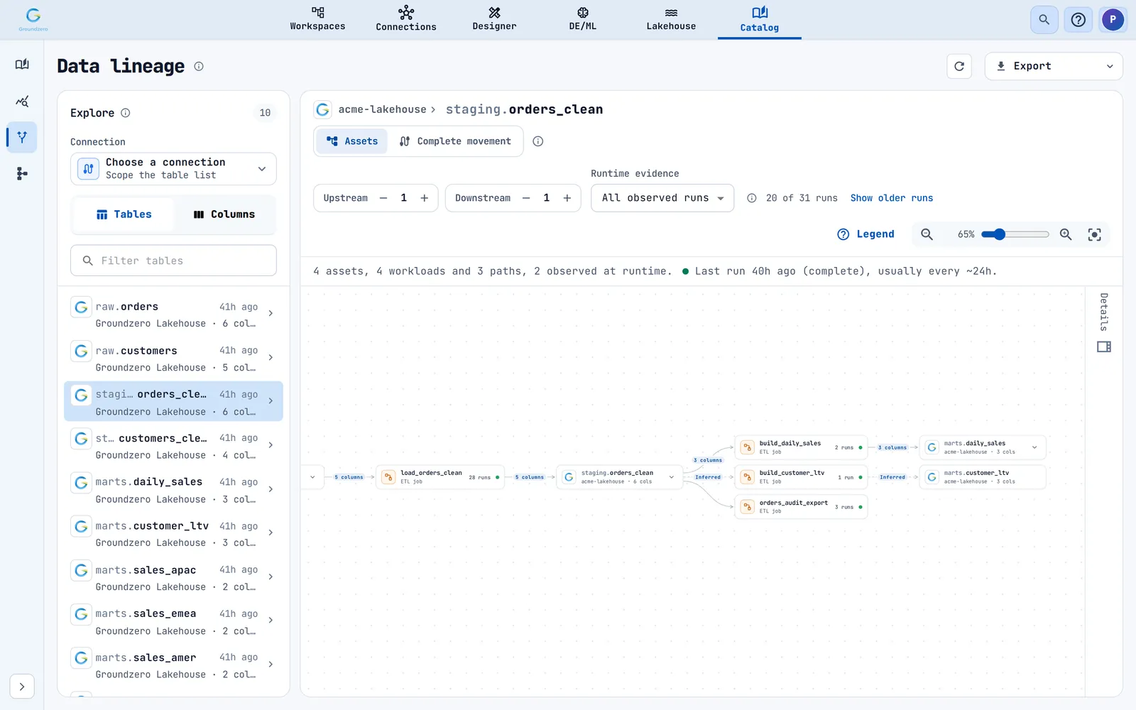
What you should see: The table you chose, with the job that writes it on one side and the jobs and tables that read it on the other.
Use lineage before you change something
Before you rename a column or retire a table, open its lineage and its Impact tab to see the jobs and tables that depend on it.
If something goes wrong: If the page says Choose a table to trace, pick a connection and then a table.
What you built#
You have now used every main area of Groundzero.
| Step | Where | What you made |
|---|---|---|
| 1 | Connections | A saved link to a data source |
| 2 | Catalog | A description and tags on what you found |
| 3 | Designer, Datasets | A named SQL dataset |
| 4 | Designer, Visualizations | A chart on that dataset |
| 5 | Designer, Dashboards; Workspaces | A published dashboard in a workspace |
| 6 | DE/ML | A project, a job and a daily schedule |
| 7 | Catalog, Data Lineage | A map of how it fits together |